Quantile plot of time series

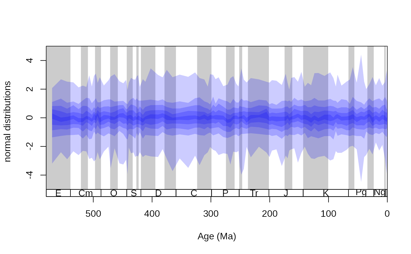
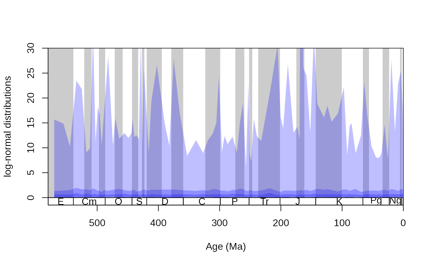
This intermediate-level function will plot a time series with the quantiles shown with transparency values.

Usage

shades(
  x,
  y,
  col = "black",
  res = 10,
  border = NA,
  interpolate = FALSE,
  method = "symmetric",
  na.rm = FALSE
)

Arguments

x

(numeric): The x coordinates.

y

(numeric matrix): The series of distributions to be plotted. Every row represents a distribution of values. The number of rows must equal to the length of x.

col

(character): The color of the quantiles, currently just a single color is allowed.

res

(numeric): If a single value is entered, than this argument represents the number of quantiles to be shown (coerced to 150, if higher is entered). If it is vector of values, it will be interpreted as the vector of quantiles to be shown. If method="symmetric", only an odd number of quantiles are plotted.

border

(character): The color of the quantile lines. A single value, by default, no lines are drawn (border=NA).

interpolate

(logical): In case the symmetric method is chosen, the series of quantile values can be interpolated with a LOESS function.

method

(character): The default "symmetric" method will plot the mid quantile range with highest opacity and the shades will be more translucent at the tails of the distributions. The "decrease" method will decrease the opacity with higher quantiles, which can make more sense for bottom-bounded distributions (e.g. exponential).

na.rm

(logical): If set to FALSE, than rows that are missing from the dataset will be plotted as gaps in the shading. If set to TRUE, than these gaps will be skipped.

Value

The function has no return value.

Examples

# some random values accross the Phanerozoic
data(stages)
tsplot(stages, boxes="sys", shading="series", ylim=c(-5,5), ylab=c("normal distributions"))
  randVar <- t(sapply(1:95, FUN=function(x){rnorm(150, 0,1)}))
  shades(stages$mid, randVar, col="blue", res=10,method="symmetric")

  
# a bottom-bounded distribution (log normal)
tsplot(stages, boxes="sys", shading="series", ylim=c(0,30), ylab="log-normal distributions")
  randVar <- t(sapply(1:95, FUN=function(x){rlnorm(150, 0,1)}))
  shades(stages$mid, randVar, col="blue", res=c(0,0.33, 0.66, 1),method="decrease")